CASSI
⬡ MAINNETCoded Aperture Snapshot Spectral Imaging
This imaging system is live on mainnet
Solutions submitted here earn real PWM. Submit a reconstruction solution or contribute a benchmark to start mining rewards.
Standard reconstruction benchmark — forward model perfectly known, no calibration needed. Score = 0.5 × clip((PSNR−15)/30, 0, 1) + 0.5 × SSIM
| # | Method | Score | PSNR (dB) | SSIM | Source | |
|---|---|---|---|---|---|---|
| 🥇 | MiJUN-5stg | 0.927 | 40.9 | 0.991 | ✓ Certified | Meng et al. AAAI 2025 |
| 🥈 | RDLUF-MixS2-9stg | 0.904 | 39.6 | 0.988 | ✓ Certified | Dong et al. CVPR 2023 |
| 🥉 | DAUHST-9stg | 0.883 | 38.4 | 0.985 | ✓ Certified | Cai et al. NeurIPS 2022 |
| 4 | PADUT-3stg | 0.854 | 36.95 | 0.975 | ✓ Certified | Li et al. ICCV 2023 |
| 5 | CST-L-Plus | 0.836 | 36.1 | 0.967 | ✓ Certified | Cai et al. ECCV 2022 |
| 6 | MST++ | 0.833 | 36.0 | 0.966 | ✓ Certified | Cai et al. CVPRW 2022 |
| 7 | MST-L | 0.809 | 34.81 | 0.958 | ✓ Certified | Cai et al. CVPR 2022 |
| 8 | HDNet | 0.804 | 34.66 | 0.952 | ✓ Certified | Hu et al. CVPR 2022 |
| 9 | SSR-L | 0.797 | 34.0 | 0.960 | ✓ Certified | Zhang et al. CVPR 2024 |
| 10 | DGSMP | 0.752 | 32.6 | 0.917 | ✓ Certified | Huang et al. CVPR 2021 |
| 11 | TSA-Net | 0.722 | 31.5 | 0.894 | ✓ Certified | Meng et al. ECCV 2020 |
| 12 | λ-Net | 0.696 | 30.1 | 0.887 | ✓ Certified | Miao et al. ICCV 2019 |
| 13 | BIRNAT | 0.694 | 30.0 | 0.887 | ✓ Certified | Cheng et al. ECCV 2022 |
| 14 | ADMM-Net | 0.674 | 29.1 | 0.877 | ✓ Certified | Ma et al. ICCV 2019 |
| 15 | GAP-Net | 0.669 | 29.1 | 0.867 | ✓ Certified | Meng et al. 2020 |
| 16 | GAP-TV | 0.577 | 24.34 | 0.820 | ✓ Certified | Yuan et al. 2016 |
|
Per-scene breakdown — KAIST 10-scene test set (PWM run, FISTA+TV, 100 iter)
scene01
24.63 dB
0.6848
scene02
19.87 dB
0.5263
scene03
22.94 dB
0.7450
scene04
31.82 dB
0.8719
scene05
21.59 dB
0.6472
scene06
22.26 dB
0.6586
scene07
17.78 dB
0.5688
scene08
22.77 dB
0.6745
scene09
23.06 dB
0.6953
scene10
23.50 dB
0.5709
avg
23.02 dB
0.6643
|
||||||
| 17 | PnP-HSICNN | 0.573 | 25.12 | 0.810 | ✓ Certified | Maffei et al. 2020 |
| 18 | TwIST | 0.538 | 23.1 | 0.800 | ✓ Certified | Bioucas-Dias & Figueiredo 2007 |
Dataset: KAIST simu, 256×256×28
Blind Reconstruction Challenge — forward model has unknown mismatch, must calibrate from data. Score = 0.4 × PSNR_norm + 0.4 × SSIM + 0.2 × (1 − ‖y − Ĥx̂‖/‖y‖)
| # | Method | Overall Score | Public PSNR / SSIM |
Dev PSNR / SSIM |
Hidden PSNR / SSIM |
Trust | Source |
|---|---|---|---|---|---|---|---|
| 🥇 | SSR-L + gradient | 0.626 |
0.877
38.03 dB / 0.994
|
0.545
19.53 dB / 0.626
|
0.456
17.06 dB / 0.473
|
✓ Certified | PWM benchmark (CVPR 2024) |
| 🥈 | GAP-TV + gradient | 0.593 |
0.687
24.21 dB / 0.865
|
0.576
19.69 dB / 0.699
|
0.516
18.37 dB / 0.583
|
✓ Certified | PWM benchmark |
| 🥉 | MST-L + gradient | 0.550 |
0.794
31.29 dB / 0.977
|
0.472
17.18 dB / 0.550
|
0.385
15.45 dB / 0.384
|
✓ Certified | PWM benchmark |
| 4 | PnP-HSICNN + gradient | 0.504 |
0.549
20.06 dB / 0.675
|
0.508
16.88 dB / 0.621
|
0.455
15.59 dB / 0.518
|
✓ Certified | PWM benchmark |
| 5 | HDNet + gradient | 0.439 |
0.707
25.45 dB / 0.921
|
0.329
13.59 dB / 0.427
|
0.280
10.96 dB / 0.373
|
✓ Certified | PWM benchmark |
Complete score requires all 3 tiers (Public + Dev + Hidden).
Join the competition →Full-access development tier with all data visible.
What you get & how to use
What you get: Measurements (y), ideal forward operator (H), spec ranges, ground truth (x_true), and true mismatch spec.
How to use: Load HDF5 → compare reconstruction vs x_true → check consistency → iterate.
What to submit: Reconstructed signals (x_hat) and corrected spec as HDF5.
Public Leaderboard
| # | Method | Score | PSNR | SSIM |
|---|---|---|---|---|
| 1 | SSR-L + gradient | 0.877 | 38.03 | 0.994 |
| 2 | MST-L + gradient | 0.794 | 31.29 | 0.977 |
| 3 | HDNet + gradient | 0.707 | 25.45 | 0.921 |
| 4 | GAP-TV + gradient | 0.687 | 24.21 | 0.865 |
| 5 | PnP-HSICNN + gradient | 0.549 | 20.06 | 0.675 |
Spec Ranges (5 parameters)
| Parameter | Min | Max | Unit |
|---|---|---|---|
| mask_dx | 0.3 | 0.7 | px |
| mask_dy | 0.1 | 0.5 | px |
| mask_rotation | 0.0 | 0.2 | deg |
| dispersion_slope | 1.895 | 2.145 | px/band |
| dispersion_axis | 0.0 | 0.3 | deg |
Blind evaluation tier — no ground truth available.
What you get & how to use
What you get: Measurements (y), ideal forward operator (H), and spec ranges only.
How to use: Apply your pipeline from the Public tier. Use consistency as self-check.
What to submit: Reconstructed signals and corrected spec. Scored server-side.
Dev Leaderboard
| # | Method | Score | PSNR | SSIM |
|---|---|---|---|---|
| 1 | GAP-TV + gradient | 0.576 | 19.69 | 0.699 |
| 2 | SSR-L + gradient | 0.545 | 19.53 | 0.626 |
| 3 | PnP-HSICNN + gradient | 0.508 | 16.88 | 0.621 |
| 4 | MST-L + gradient | 0.472 | 17.18 | 0.55 |
| 5 | HDNet + gradient | 0.329 | 13.59 | 0.427 |
Spec Ranges (5 parameters)
| Parameter | Min | Max | Unit |
|---|---|---|---|
| mask_dx | 0.4 | 0.8 | px |
| mask_dy | 0.2 | 0.6 | px |
| mask_rotation | 0.05 | 0.25 | deg |
| dispersion_slope | 1.825 | 2.075 | px/band |
| dispersion_axis | 0.07 | 0.37 | deg |
Fully blind server-side evaluation — no data download.
What you get & how to use
What you get: No data downloadable. Algorithm runs server-side on hidden measurements.
How to use: Package algorithm as Docker container / Python script. Submit via link.
What to submit: Containerized algorithm accepting y + H, outputting x_hat + corrected spec.
Hidden Leaderboard
| # | Method | Score | PSNR | SSIM |
|---|---|---|---|---|
| 1 | GAP-TV + gradient | 0.516 | 18.37 | 0.583 |
| 2 | SSR-L + gradient | 0.456 | 17.06 | 0.473 |
| 3 | PnP-HSICNN + gradient | 0.455 | 15.59 | 0.518 |
| 4 | MST-L + gradient | 0.385 | 15.45 | 0.384 |
| 5 | HDNet + gradient | 0.280 | 10.96 | 0.373 |
Spec Ranges (5 parameters)
| Parameter | Min | Max | Unit |
|---|---|---|---|
| mask_dx | 0.2 | 0.6 | px |
| mask_dy | 0.0 | 0.4 | px |
| mask_rotation | -0.05 | 0.15 | deg |
| dispersion_slope | 1.955 | 2.205 | px/band |
| dispersion_axis | -0.05 | 0.25 | deg |
Blind Reconstruction Challenge
ChallengeGiven measurements with unknown mismatch and spec ranges (not exact params), reconstruct the original signal. A method must be evaluated on all three tiers for a complete score. Scored on a composite metric: 0.4 × PSNR_norm + 0.4 × SSIM + 0.2 × (1 − ‖y − Ĥx̂‖/‖y‖).
Measurements y, ideal forward model H, spec ranges
Reconstructed signal x̂
About the Imaging Modality
CASSI captures a 3D hyperspectral data cube (2 spatial + 1 spectral dimension) in a single 2D camera exposure. The scene is modulated by a binary coded aperture mask, spectrally dispersed by a prism, and integrated onto a 2D detector. The forward model is y = H*x + n where H encodes both coded-aperture modulation and spectral-dispersion shift. Compression ratios equal the number of spectral bands (e.g. 28:1). Reconstruction exploits spectral correlation via GAP-TV, MST, or CST.
Principle
Coded Aperture Snapshot Spectral Imaging (CASSI) captures a full 3-D spectral datacube (x, y, λ) in a single 2-D snapshot by encoding the scene with a binary coded aperture and spectrally dispersing it with a prism onto the detector. Different spectral channels are shifted and superimposed on the sensor, creating a compressed measurement. Computational algorithms recover the full datacube from this single measurement using sparsity priors.
How to Build the System
Build an optical relay with an objective lens, place a binary coded aperture (lithographic chrome-on-glass mask or DMD) at an intermediate image plane, then disperse with an Amici or double-Amici prism, and re-image onto a high-resolution detector (2048× 2048+ pixels). Precisely calibrate the spectral dispersion curve (nm/pixel). The coded aperture pattern should have ~50 % transmittance and good conditioning.
Common Reconstruction Algorithms
- TwIST (Two-step Iterative Shrinkage/Thresholding)
- GAP-TV (Generalized Alternating Projection with Total Variation)
- ADMM with sparsity in DCT or wavelet domain
- Deep unfolding networks (DGSMP, TSA-Net, BIRNAT)
- Plug-and-Play ADMM with learned denoisers
Common Mistakes
- Poor spectral calibration causing wavelength assignment errors across the datacube
- Coded aperture not precisely at the image plane, blurring the code modulation
- Insufficient detector resolution relative to the number of spectral bands
- Ignoring optical aberrations in the dispersive relay that vary with wavelength
- Using a random mask without checking its sensing matrix condition number
How to Avoid Mistakes
- Calibrate spectral mapping with monochromatic sources at known wavelengths
- Mount coded aperture on a precision z-stage and focus to maximize modulation contrast
- Ensure detector pixel count > (spatial pixels × spectral bands) for adequate compression ratio
- Design the relay optics for uniform imaging quality across the spectral range
- Optimize or simulate the mask pattern for low coherence (good RIP) before fabrication
Forward-Model Mismatch Cases
- The widefield fallback produces a 2D (64,64) grayscale image, but CASSI compresses a 3D spectral datacube (64,64,L wavelengths) into a single 2D coded snapshot via a binary mask and dispersive prism — the spectral dimension is entirely absent
- Without the coded aperture mask and spectral dispersion, the measurement does not encode wavelength-dependent information — spectral unmixing or hyperspectral reconstruction from the fallback output is impossible
How to Correct the Mismatch
- Use the CASSI operator that applies the binary coded aperture mask followed by spectral dispersion (prism/grating shift), producing a 2D coded measurement that encodes the full 3D spectral datacube
- Reconstruct the (x,y,lambda) datacube using compressive sensing (TwIST, GAP-TV) or deep unfolding networks (TSA-Net, MST) that exploit the spatio-spectral structure encoded by the CASSI forward model
Experimental Setup — Signal Chain

Reconstruction Gallery — 4 Scenes × 3 Scenarios
Method: CPU_baseline | Mismatch: nominal (nominal=True, perturbed=False)
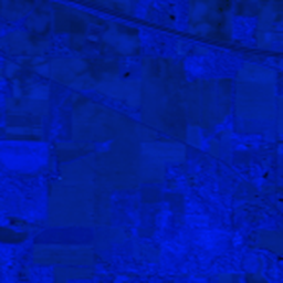
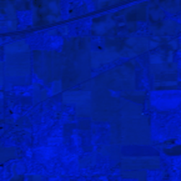
Ground Truth

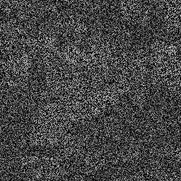
Measurement
Reconstruction
Ground Truth

Measurement
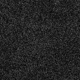
Reconstruction
Ground Truth
Measurement (perturbed)
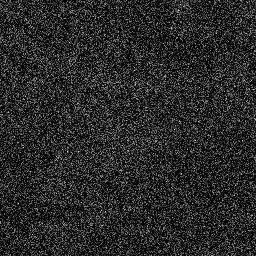
Reconstruction


Mean PSNR Across All Scenes
Per-scene PSNR breakdown (4 scenes)
| Scene | I (PSNR) | I (SSIM) | II (PSNR) | II (SSIM) | III (PSNR) | III (SSIM) |
|---|---|---|---|---|---|---|
| scene_00 | 11.388157370414833 | 0.01733572164482545 | 16.29034469671149 | 0.04138063796264847 | 16.419408068168842 | 0.045509048931950055 |
| scene_01 | 11.604006893341834 | 0.01871242508822704 | 16.262318979148382 | 0.041985050757947055 | 16.342202770675012 | 0.045774250082260305 |
| scene_02 | 11.332959495650615 | 0.01710600322887299 | 16.354152003784925 | 0.043263103647925995 | 16.27598154571157 | 0.04582825340291557 |
| scene_03 | 11.9781210538936 | 0.01968244532966781 | 16.251118459587204 | 0.04159571449035334 | 16.38499506997022 | 0.04578811472898349 |
| Mean | 11.575811203325221 | 0.018209148822898324 | 16.289483534808 | 0.042056126714718714 | 16.35564686363141 | 0.04572491678652736 |
Experimental Setup
Key References
- Wagadarikar et al., 'Single disperser design for coded aperture snapshot spectral imaging', Applied Optics 47, B44-B51 (2008)
- Cai et al., 'Mask-guided Spectral-wise Transformer (MST++)', CVPRW 2022
Canonical Datasets
- CAVE (Columbia, 32 scenes, 512x512x31)
- KAIST (30 scenes, 2704x3376x28)
- ARAD_1K (1000 hyperspectral images)
Spec DAG — Forward Model Pipeline
M(mask) → W(α, a) → Σ_λ → D(g, η₄)
Mismatch Parameters
| Symbol | Parameter | Description | Nominal | Perturbed |
|---|---|---|---|---|
| Δx | mask_dx | Mask lateral shift (pixels) | 0 | 0.5 |
| Δy | mask_dy | Mask vertical shift (pixels) | 0 | 0.3 |
| θ | mask_theta | Mask rotation (rad) | 0 | 0.1 |
| a₁ | disp_a1 | Dispersion coefficient | 2.0 | 2.02 |
| α | disp_alpha | Dispersion angle (rad) | 0 | 0.15 |
| σ_r | sigma_read | Detector read noise std (electrons) | 5.0 | 8.0 |
| I_d | dark_current | Dark current (electrons/pixel/s) | 0.1 | 0.5 |
| g | gain | Detector gain multiplier | 1.0 | 1.03 |
Credits System
Spec Primitives Reference (11 primitives)
Free-space or medium propagation kernel (Fresnel, Rayleigh-Sommerfeld).
Spatial or spatio-temporal amplitude modulation (coded aperture, SLM pattern).
Geometric projection operator (Radon transform, fan-beam, cone-beam).
Sampling in the Fourier / k-space domain (MRI, ptychography).
Shift-invariant convolution with a point-spread function (PSF).
Summation along a physical dimension (spectral, temporal, angular).
Sensor readout with gain g and noise model η (Gaussian, Poisson, mixed).
Patterned illumination (block, Hadamard, random) applied to the scene.
Spectral dispersion element (prism, grating) with shift α and aperture a.
Sample or gantry rotation (CT, electron tomography).
Spectral filter or monochromator selecting a wavelength band.